
Empirical Rule:Since gathering the appropriate data may be time-consuming or even impossible in some cases, this probability distribution can be used as an interim heuristic in the meantime. In reviewing quality control measures or evaluating risk exposure, a firm has to take such considerations into account. VaR, a risk assessment tool often used in financial planning, assumes the probability of risk events follows a normal distribution.
Additionally, the empirical rule is used as a rough guide to determine a distribution’s “normality.” If too many data points are outside the three standard deviation boundaries, the distribution may not be normal and may be skewed or follow some other distribution.
The three-sigma rule is also called the bell curve rule, since it refers to a data distribution that is within three standard deviations of the average.
Empirical Rule
According to the empirical rule, also known as the three-sigma rule or the 68-95-99.7 rule, almost all observed data will fall between three standard deviations of the mean or average.
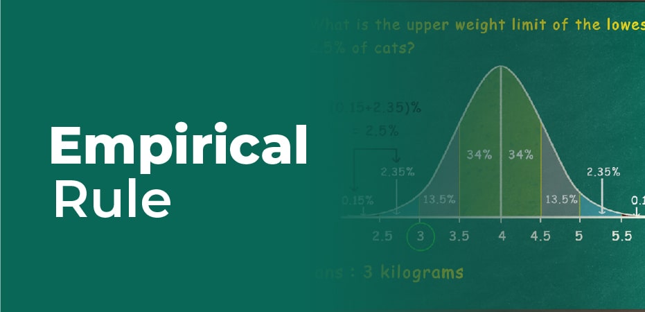
In particular, the empirical rule foretells that 68% of observations falls within the first standard deviation (µ ± σ), 95% within the first two standard deviations (µ ± 2σ), and 99.7% within the initial three standard deviations (µ ± 3σ).
History
In 1733, Abraham de Moivre proposed the 68 95 99.7 rule, 75 years before the normal distribution model was published. De Moivre worked in the burgeoning field of probability. Perhaps his most significant contribution to statistics is in the 1756 edition of The Doctrine of Chances, which applied the normal distribution as an approximation for binomial distribution when many trials were available.
An experiment by De Moivre led to the discovery of the 68 95 99.7 rule. You can do your experiment by flipping 100 fair coins. Note:
- In this binomial experiment, you would expect to see a certain number of heads.
- The standard deviation.
- Sixty-eight percent of the time, ninety-five percent of the time, and 99.7% of the time, you would get the same number of heads
Normal distribution
The empirical rule came about because the exact shape of distribution curves continued to appear repeatedly to statisticians. A normal distribution can be described by the empirical rule. The standard deviation of a normal distribution is generally between three and five standard deviations. This is also true for the mode and median.
- All the numbers in the data set are averaged to generate the mean.
- The mode is the number that repeats most frequently in the data set.
- A median is defined as the value of the spread between the highest and lowest numbers within a set.
This means that the mean, mode, and median should all fall at the center of the dataset. One-half of the data should be at the higher end of the set and the other half at the lower end.

Determining the Standard Deviation
The empirical rule is specifically helpful for forecasting outcomes within a data set. It’s first necessary to determine the standard deviation.
The complicated formula breaks down in the following way:
- Determine the mean of the data set, which is the total of the data set divided by the number of numbers.
- Subtract the mean from every number, then square the result.
- Calculate the means from the squared values.
- Calculate the square root of the means calculated in step 3.
That is the standard deviation of the normal distribution between its three primary percentages. Including a very small percentage of outliers, the majority of the data should fall into this range.
Using the Empirical Rule
As mentioned above, the empirical rule is beneficial for forecasting outcomes within a data set. When the standard deviation has been determined, the data set can easily be subjected to the empirical rule, which shows where the pieces of data lie within the distribution.
Without knowing all the specifics of data, projections can be made about where data will fall based on the 68%, 95%, and 99.7% guidelines that specify where all data should rest.
In most cases, the empirical rule is primarily used to help determine outcomes when not all the data is available. Those who study statistics – or the data – can gain insight into where all of the data will fall once it is available. Ethical rules are also valuable in testing the normality of data sets. Data that does not follow the empirical rule is not a normal distribution and must be calculated accordingly.
FAQs
What Is the Empirical Rule?
Statistics states that 99.7% of data falls within three standard deviations of the mean within a normal distribution. Thus, 68.3% of the observed data will fall within the first standard deviation, 95% within the second deviation, and 97.3% within the third standard deviation. These statistics give us a rough idea of how a probability distribution will turn out.
How Is the Empirical Rule Used?
To predict probable outcomes under a normal distribution, the empirical rule is applied. This would be useful to a statistician when estimating the percentage of cases within a standard deviation. If the standard deviation was 3.1 and the mean was 10, then this would be useful. In this case, the first standard deviation is between (10+3.2)= 13.2 and (10-3.2)= 6.8. The second standard deviation is between (10 + 2×3.2)= 16.4 and 10 – (2×3.2)= 3.6, and so on.
What Are the Benefits of the Empirical Rule?
Data can be forecasted using the empirical rule, as it serves as an efficient method for forecasting. It is particularly true when it comes to large datasets and variables that are unknown. In finance specifically, the empirical rule is pertinent to stock prices, price indices, and log values of forex rates, which tend to fall across a bell curve or normal distribution.